How to: Poisson Regression Model + Python Implementation

As my first post I'll be attempting to make almost the whole inference of the Poisson regression model, which is also a course work for my class of Pattern recognition, so don't try this at home.

In this post we will cover:

What is the Poisson Regression?
The Poisson Distribution as part of the Exponential Family
Maximum Log-Likelihood method
Derivating the $loss$ function
The matricial representation
A simple implementation
Awesome references

1. What is the Poisson Regression?

We already know about the Linear Regression, which helps us answer questions like "How much will a house with these characteristics cost?". Or the Logistic Regression, which is used to model the probability of a certain class or event existing such as pass/fail, win/lose, alive/dead or healthy/sick.

But, what happens when the questions are "How many costumers will come today?", "How many people are in line at the grocery store?", "How many...?", and one way to answer these questions is using the Poisson Regression Model.

Poisson Regression is used to model count data. For this, we assume the response variable $Y$ has a Poisson Distribution, and assumes the logarithm of its expected value can be modeled by a linear combinations of unknown parameters.

2. The Poisson Distribution as part of the Exponential Family

Alright, first things first, can we express the Poisson distribution on the Exponential Family form? Well, we can find that out.
First, if we have a random variable $X$ such that \[X\sim ExpFam(\theta)\] we know we can express its probability function as the following \begin{equation} P_X(X=x\ | \ \theta) = h(x) e^{\eta(\theta)T(x) - A(\theta)} \ \ \ \ (1) \end{equation} Okay, now let's do this, assume we have a random variable $Y$ that is distributed as a Poisson with a parameter $\lambda$ \[Y\sim Poisson(\lambda)\] with its probability function being \[P_Y(Y=y \ | \ \lambda) = \frac{e^{-\lambda}\lambda^{y}}{y!}\] We know that \[ P_y(Y=y \ | \ \lambda) = \frac{e^{-\lambda}\lambda^{y}}{y!} = \\ \frac{1}{y!} e^{-\lambda}\lambda^{y} = \\ \frac{1}{y!}e^{\log(e^{-\lambda}\lambda^{y})} = \] \[ \frac{1}{y!}e^{\log(e^{-\lambda}) + \log(\lambda^{y})} = \\ \frac{1}{y!} e^{-\lambda + y \log(\lambda)} = \\ \frac{1}{y!} e^{y \log(\lambda) - \lambda} \] and thus \begin{equation} P_y(Y=y \ | \ \lambda) = \frac{1}{y!} e^{y \log(\lambda) - \lambda} \ \ \ \ (2) \end{equation} but wait a minute, the equation $(2)$ has the same form as the equation $(1)$ ! \[\theta = \lambda\] \[h(y) = \frac{1}{y!}\] \[\eta(\lambda) = \log(\lambda)\] \[T(y) = y\] \[A(\lambda) = \lambda\] and thus \begin{equation} P_Y(Y=y \ | \ \lambda) = h(y) e^{\eta(\lambda)T(y) - A(\lambda)} \ \ \ \ (3) \end{equation} Finally we can say \[Y \sim ExpFam(\lambda)\]

3. Maximum Log-Likelihood method

Okay! Now, assume we have a random variable $Y$ such as \[ Y \sim Poisson(\lambda) \] and for $(3)$ we now we can express its probability function as \[ P_Y(Y=y | \lambda) = h(y) e^{\eta(\lambda)T(y) - A(\lambda)} \] Recall \[\eta(\lambda) = \log(\lambda) \Rightarrow \lambda = e^\eta\] and we do know for GLM that \[\eta = w^\intercal x + b \] and thus \begin{equation} \lambda = e^{w^\intercal x + b} \ \ \ \ (4) \end{equation} Alright, now if we have a set of $m$ observations \[\{(x^{(1)}, y^{(1)}), (x^{(2)}, y^{(2)}), \ldots , (x^{(m)}, y^{(m)})\}\] where we assume for each $y^{(i)}$ being $i.i.d.$ and we are looking to maximize the following probability function \[ P_Y[y^{(1)}, y^{(2)}, \dots, y^{(m)} \ | \ x^{(1)}, x^{(2)}, \dots, x^{(m)}] \\ = \prod_{i = 1}^{m} h(y^{(i)}) e^{\eta(\lambda^{(i)})T(y^{(i)}) - A(\lambda^{(i)})} \] Now we use our secret ~~not so secret~~ weapon, the Maximum Likelihood method \[ w^*, b^* = arg\max_{w \in \mathbb{R}^n, \ b \in \mathbb{R}} \prod_{i = 1}^{m} h(y^{(i)}) e^{\eta(\lambda^{(i)})T(y^{(i)}) - A(\lambda^{(i)})} \] \[ w^*, b^* = arg\max_{w \in \mathbb{R}^n, \ b \in \mathbb{R}} \prod_{i = 1}^{m} \frac{1}{y^{(i)}!} e^{\log(\lambda^{(i)})y^{(i)} - \lambda^{(i)}} \] and for the Maximum Log-Likelihood method \[ w^*, b^* = arg\max_{w \in \mathbb{R}^n, \ b \in \mathbb{R}} \sum_{i = 1}^{m} \log(\frac{1}{y^{(i)}!} e^{\log(\lambda^{(i)})y^{(i)} - \lambda^{(i)}}) \] \[ w^*, b^* = arg\max_{w \in \mathbb{R}^n, \ b \in \mathbb{R}} \sum_{i = 1}^{m} \log(\frac{1}{y^{(i)}!}) + \log(e^{\log(\lambda^{(i)})y^{(i)} - \lambda^{(i)}}) \] since $\log(\frac{1}{y!})$ does not depend on $w^*$ or $b^*$ \[ w^*, b^* = arg\max_{w \in \mathbb{R}^n, \ b \in \mathbb{R}} \sum_{i = 1}^{m} \log(e^{\log(\lambda^{(i)})y^{(i)} - \lambda^{(i)}}) \] \[ w^*, b^* = arg\max_{w \in \mathbb{R}^n, \ b \in \mathbb{R}} \sum_{i = 1}^{m} \log(\lambda^{(i)})y^{(i)} - \lambda^{(i)} \] and since we would like to minimize instead of maximize \[ w^*, b^* = arg\min_{w \in \mathbb{R}^n, \ b \in \mathbb{R}} \sum_{i = 1}^{m} \lambda^{(i)} - \log(\lambda^{(i)})y^{(i)} \] but we know \begin{equation} y \sim Poisson(\lambda) \Rightarrow \\ E[y] = \lambda = \hat{y} = e^{\eta} = e^{w^\intercal x + b} \ \ \ \ (5) \end{equation} and thus \[ w^*, b^* = arg\min_{w \in \mathbb{R}^n, \ b \in \mathbb{R}} \sum_{i = 1}^{m} \hat{y}^{(i)} - \log(\hat{y}^{(i)})y^{(i)} \] and because we want an average \[ w^*, b^* = arg\min_{w \in \mathbb{R}^n, \ b \in \mathbb{R}} \frac{1}{m} \sum_{i = 1}^{m} \hat{y}^{(i)} - \log(\hat{y}^{(i)})y^{(i)} \] finally obtaining the following $loss$ function \begin{equation} loss = \frac{1}{m} \sum_{i = 1}^{m} \hat{y}^{(i)} - \log(\hat{y}^{(i)})y^{(i)} \ \ \ \ (6) \end{equation}

4. Derivating the $loss$ function

Now that we have a $loss$ function, we want it to have a value as low as possible, so we do what we learned on high school and derivate to find the minimum. First we do it respect our vector of features $w$ and make it equal to $0$ \[ \frac{\partial}{\partial w} loss = 0 \] and for $(5)$ and $(6)$ we have \[ loss = \frac{1}{m} \sum^{m}_{i=1} e^{w^\intercal x^{(i)} + b} - (w^\intercal x^{(i)} + b)y^{(i)} \] and thus \[ \frac{\partial}{\partial w} loss = \frac{\partial}{\partial w} \frac{1}{m} \sum^{m}_{i=1} e^{w^\intercal x^{(i)} + b} - (w^\intercal x^{(i)} + b)y^{(i)} \] \[ \frac{\partial}{\partial w} loss = \frac{1}{m} \sum^{m}_{i=1} x^{(i)}e^{w^\intercal x^{(i)} + b} - x^{(i)})y^{(i)} \] \[ \frac{\partial}{\partial w} loss = \frac{1}{m} \sum^{m}_{i=1} x^{(i)}(e^{w^\intercal x^{(i)} + b} - y^{(i)}) \] \begin{equation} \frac{\partial}{\partial w} loss = \frac{1}{m} \sum^{m}_{i=1} x^{(i)}(\hat{y}^{(i)} - y^{(i)}) \ \ \ \ (7) \end{equation} and we do the same for $b$ \[ \frac{\partial}{\partial b} loss = \frac{\partial}{\partial b} \frac{1}{m} \sum^{m}_{i=1} e^{w^\intercal x^{(i)} + b} - (w^\intercal x^{(i)} + b)y^{(i)} \] \[ \frac{\partial}{\partial b} loss = \frac{1}{m} \sum^{m}_{i=1} e^{w^\intercal x^{(i)} + b} - y^{(i)} \] \begin{equation} \frac{\partial}{\partial b} loss = \frac{1}{m} \sum^{m}_{i=1} \hat{y}^{(i)} - y^{(i)} \ \ \ \ (8) \end{equation}

5. The matricial representation

We're almost there! Now, we know we can represent the information of our observations as the following \begin{equation*} X = \begin{pmatrix} x^{(1)}_1 & x^{(1)}_2 & \cdots & x^{(1)}_n \\ x^{(2)}_1 & x^{(2)}_2 & \cdots & x^{(2)}_n \\ \vdots & \vdots & \ddots & \vdots \\ x^{(m)}_1 & x^{(m)}_2 & \cdots & x^{(m)}_n \end{pmatrix} \ \ \ \ \ \ \ \\ Y = \begin{pmatrix} y^{(1)}_1 \\ y^{(2)}_1 \\ \vdots \\ y^{(m)}_1 \end{pmatrix} \end{equation*} and we also have a feature vector $w$ and a bias vector $\vec{b}$ \begin{equation*} w = \begin{pmatrix} w_1 \\ w_2 \\ \vdots \\ w_n \end{pmatrix} \ \ \ \ \ \ \ \vec{b} = \begin{pmatrix} b \\ b \\ \vdots \\ b \end{pmatrix} \end{equation*} Now let's define a matrix $Z$ such that $$ Z = Xw + \vec{b} = \\ \begin{pmatrix} x^{(1)}_1 & x^{(1)}_2 & \cdots & x^{(1)}_n \\ x^{(2)}_1 & x^{(2)}_2 & \cdots & x^{(2)}_n \\ \vdots & \vdots & \ddots & \vdots \\ x^{(m)}_1 & x^{(m)}_2 & \cdots & x^{(m)}_n \end{pmatrix} \begin{pmatrix} w_1 \\ w_2 \\ \vdots \\ w_n \end{pmatrix} + \begin{pmatrix} b \\ b \\ \vdots \\ b \end{pmatrix} $$ and a function $\sigma$ as the following $$ \sigma(z^{(i)}) = e^{z^{(i)}} $$ and now we do \[ \sigma(Z) = \begin{pmatrix} \sigma(z^{(1)}) \\ \sigma(z^{(2)}) \\ \vdots \\ \sigma(z^{(m)}) \\ \end{pmatrix} \] where we declare a matrix $A$ that \[ A = \sigma(Z) \] and we now for $(7)$ and $(8)$ \[ \nabla w = \frac{1}{m} \sum^{m}_{i=1} x^{(i)}(\hat{y}^{(i)} - y^{(i)}) \Rightarrow \frac{1}{m} X(A - Y) \] \[ \nabla b = \frac{1}{m} \sum^{m}_{i=1} \hat{y}^{(i)} - y^{(i)} \Rightarrow \frac{1}{m} (A - Y) \]

6. A simple implementation

Alright! Now it's time to code these results, you can check out the Jupyter Notebook too see the full setup and implementation, but here I'll leave the important parts

We know that we will need the $loss$ function, so let's start with it

def loss(x, y, w, b):
  y_hat = np.exp(x @ w + b)
  error = (y_hat - np.log(y_hat) * y).mean()
  return error

Done! Let's remember we also will need to calculate the gradient with respect $w$ and also respect with $b$, down bellow I'll show you the implementation following with the gradient_descent algorithm

def grad(x, y, w, b):
  M, n = x.shape
  y_hat = np.exp(x @ w + b)
  dw = (x.T @ (y_hat - y)) / M
  db = (y_hat - y).mean()
  return dw, db

def gradient_descent(x, y, w_0, b_0, alpha, num_iter):
  w, b = w_0.copy(), b_0
  hist = np.zeros(num_iter)
  M, n = x.shape

  for iter in range(num_iter):
    dw, db = grad(x, y, w, b)
    w -= alpha * dw 
    b -= alpha * db
    hist[iter] = loss(x, y, w, b)

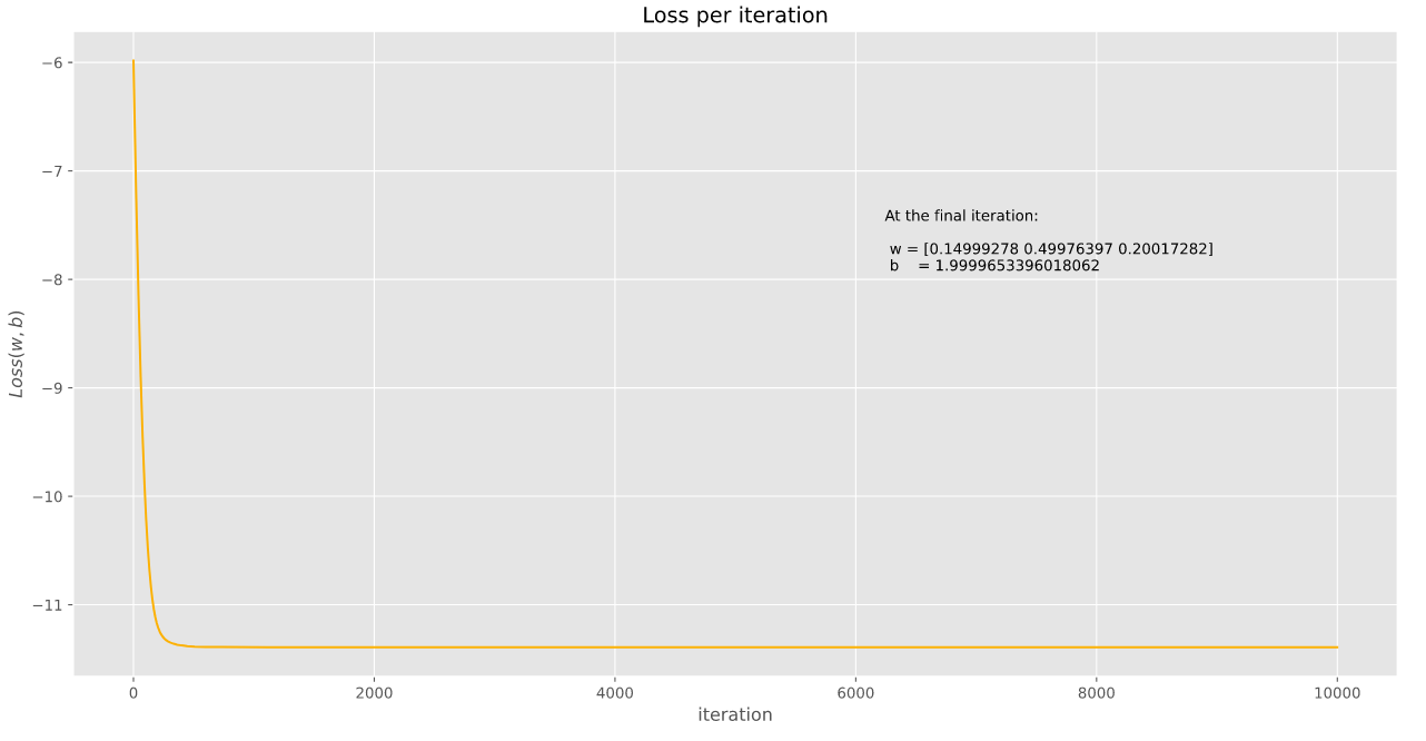
  return w, b, hist

We used these functions with a generated dataset and we calculate the following results (with the $loss$ function decreasing as we can see)

And that is pretty much it, thank you for coming to my TED Talk

via GIPHY

1. What is the Poisson Regression?

2. The Poisson Distribution as part of the Exponential Family

3. Maximum Log-Likelihood method

4. Derivating the \(loss\) function

5. The matricial representation

6. A simple implementation

7. Awesome references